
If you’re seeing the “An array value could not be found” error in Excel, you’re not alone. This common issue usually appears when a formula or function is unable to locate a specific array value within a defined range. It can be confusing, especially if your formulas seem correct on the surface.
As seasoned Excel troubleshooting experts, we’ve dealt with the “An array value could not be found” error in many real-world scenarios. Thanks to our hands-on experience, we’ve developed proven solutions that have helped thousands of users resolve this frustrating issue quickly and efficiently.
Whether you’re working with VLOOKUP, INDEX/MATCH, FILTER, or other advanced functions, we’ll walk you through exactly how to fix this error step by step.
Fix “An Array Value Could Not Be Found” Error
If you’re dealing with the “An array value could not be found” error in Excel or Google Sheets, you can resolve it efficiently by using the ARRAYFORMULA function combined with the SUBSTITUTE function. This method is especially helpful for working with multiple cells or ranges of data, making your work more efficient and less error-prone.
Follow this step-by-step guide to implement the ARRAYFORMULA with SUBSTITUTE:
🔧 Method #1: Use ARRAYFORMULA with SUBSTITUTE to Fix the Error
- Locate the cell with the SUBSTITUTE formula
First, find the cell that contains the SUBSTITUTE formula triggering the “An array value could not be found” error. - Edit the formula
Select the cell, then go to the Formula bar at the top of the window (in both Excel or Google Sheets). - Add ARRAYFORMULA to the formula
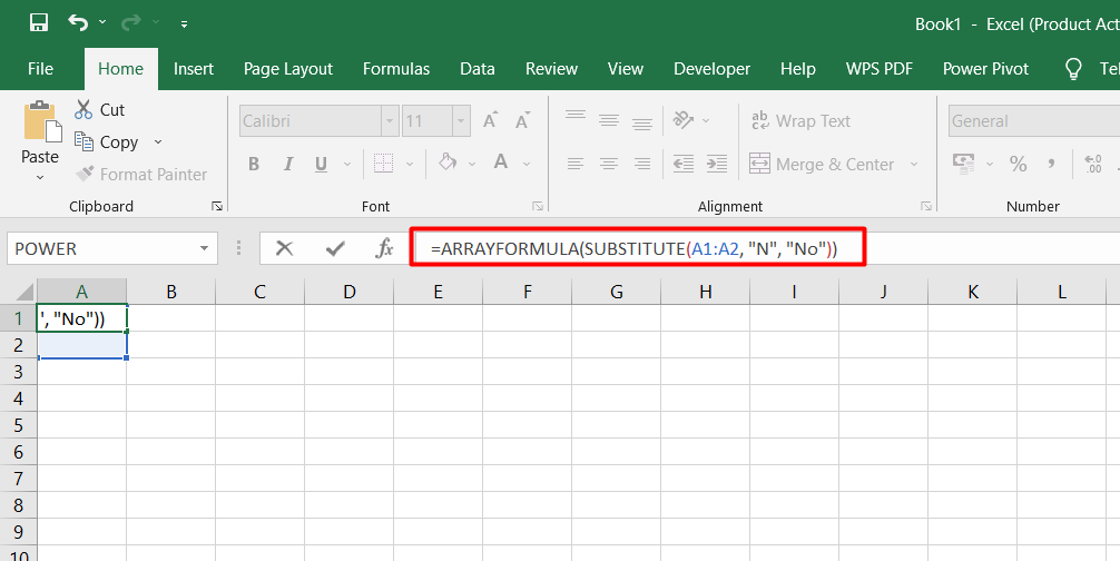
After the equal sign (=), type ARRAYFORMULA followed by an opening parenthesis. For example:=ARRAYFORMULA(SUBSTITUTE(A1:A2, "N", "No"))This tells Excel or Google Sheets to apply the SUBSTITUTE function to a range of cells (A1 to A2 in this example), avoiding the array error.
- Apply the modified formula
Press Enter to apply the new formula. By adding ARRAYFORMULA, you’re now instructing Excel or Google Sheets to handle multiple cells in one go, thus preventing the error.
✅ Why Use ARRAYFORMULA with SUBSTITUTE?
By using the ARRAYFORMULA function in combination with SUBSTITUTE, you’re simplifying the process of handling multiple cells at once. Instead of manually applying a formula to each individual cell, this method allows you to perform operations across an entire range of cells efficiently.
This technique is ideal for:
- Large datasets that require consistent operations.
- Avoiding repetitive manual inputs when working with arrays.
- Ensuring that all cells in a specified range are correctly processed.
🔧 Method #2: Use the REGEXMATCH Formula to Fix the Error
- Locate the target cell
Find the cell that you want to modify in your worksheet. - Access the Formula bar
Select the cell, then click on the Formula bar at the top of the Excel or Google Sheets window. - Enter the REGEXMATCH formula
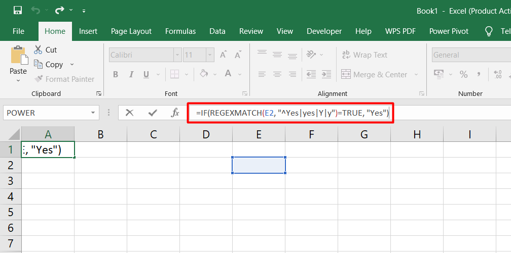
In the Formula bar, type the following formula:=IF(REGEXMATCH(E2, "^Yes|yes|Y|y")=TRUE, "Yes")This formula checks if the text in cell E2 matches any of the specified patterns (“Yes”, “yes”, “Y”, or “y”). If a match is found, it returns “Yes”.
✅ Why Use REGEXMATCH to Fix Array Errors?
The REGEXMATCH formula is incredibly useful when you need to handle text with multiple possible variations. Regular expressions (regex) give you the flexibility to search for various patterns in your data, ensuring that the formula can adapt to different text entries.
For example, you can:
- Search for different variations of Yes or No.
- Customize your search pattern to fit your specific needs, whether for text case-sensitivity or multiple word variations.
🔧 Method #3: Use REGEXREPLACE to Resolve the Error
- Select the target cell or range
Click on the cell or range of cells (e.g., B2 to B4) that you want to modify. - Access the Formula bar
Once selected, go to the Formula bar at the top of the Excel or Google Sheets window. - Enter the REGEXREPLACE formula
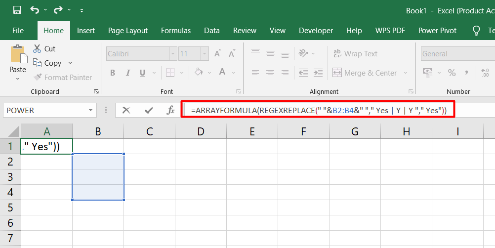
In the Formula bar, type the following formula:=ARRAYFORMULA(REGEXREPLACE(" "&B2:B4&" "," Yes | Y | y "," Yes"))This formula searches for the patterns (” Yes “, ” Y “, or ” y “) within the range (B2 to B4) and replaces them with “Yes”. The extra spaces before and after the cell values help ensure accurate pattern matching. - Apply the formula
After entering the formula, press Enter. Excel or Google Sheets will now process the specified range, replacing any instances of the specified patterns with the new text.
✅ Why Use REGEXREPLACE to Fix Array Errors?
The REGEXREPLACE function is an excellent choice when you need to perform text replacements across a range of cells. Unlike simple find-and-replace, REGEXREPLACE gives you the ability to use regular expressions for more complex matching patterns, ensuring that variations of words or phrases are handled automatically.
You can:
- Replace multiple variations of a word or phrase in a single operation.
- Customize the formula to search for any text patterns, whether exact matches or flexible variations.
- Standardize data in large datasets without manual edits.
🔧 Method #4: Combine ARRAYFORMULA with REGEXMATCH
- Select the target cell
Choose the first cell where you want to implement the formula. - Access the Formula bar
Once the cell is selected, navigate to the Formula bar at the top of the Excel or Google Sheets window. - Enter the combined formula
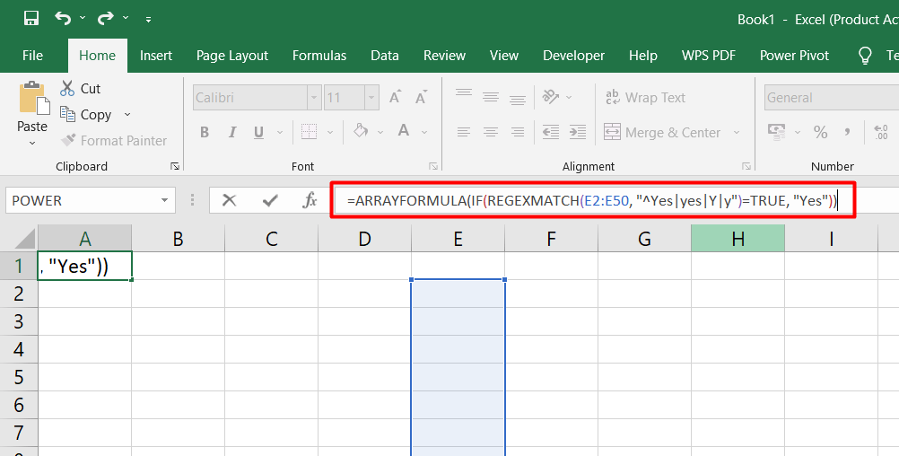
In the Formula bar, type the following formula:=ARRAYFORMULA(IF(REGEXMATCH(E2:E50, "^Yes|yes|Y|y")=TRUE, "Yes"))This formula uses REGEXMATCH to check if the text in cells E2 to E50 matches any of the patterns (“Yes”, “yes”, “Y”, or “y”). If a match is found, the formula returns “Yes” for those cells.
✅ Why Combine ARRAYFORMULA and REGEXMATCH?
By combining ARRAYFORMULA with REGEXMATCH, you’re able to perform a text match across an entire range of cells, all in one formula. This is particularly helpful when you need to apply the same operation to multiple cells without manually editing each one.
- Handle multiple cells at once: Instead of applying a formula to individual cells, ARRAYFORMULA allows you to process entire ranges of data in a single operation.
- Avoid the array error: This method prevents the “An array value could not be found” error by correctly handling multiple values and applying the function to each of them.
Conclusion
Encountering the “An array value could not be found” error in Excel or Google Sheets can be frustrating, especially when working with complex formulas or large datasets. However, with the right techniques—like using ARRAYFORMULA, REGEXMATCH, and REGEXREPLACE—you can effectively diagnose and resolve this error.
Whether you’re substituting values, matching patterns, or replacing text across multiple cells, these methods ensure your formulas function correctly and efficiently. By leveraging these advanced functions, you’ll not only fix the error but also streamline your spreadsheet workflows.
For more Excel tips, Google Sheets solutions, and formula troubleshooting guides, stay tuned to our blog. And remember—if you’re stuck, there’s always a solution just a formula away!
One more thing
If you’re in search of a software company that embodies integrity and upholds honest business practices, your quest ends here at Ecomkeys.com. As a Microsoft Certified Partner, we prioritize the trust and satisfaction of our customers. Our commitment to delivering reliable software products is unwavering, and our dedication to your experience extends far beyond the point of sale. At Ecomkeys.com, we provide a comprehensive 360-degree support system that accompanies you throughout your software journey. Your trust is our foundation, and we’re here to ensure that every interaction with us is a positive and trustworthy one.